Infrastructure requirements
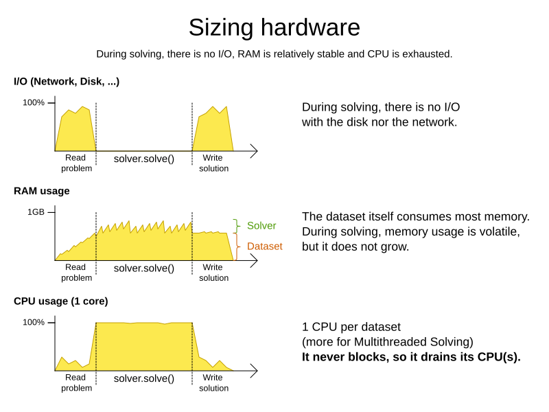
Before sizing a Timefold Solver service, first understand the typical behaviour of a Solver.solve() call:
Understand these guidelines to decide the hardware for a Timefold Solver service:
-
RAM memory: Provision plenty, but no need to provide more.
-
The problem dataset, loaded before Timefold Solver is called, often consumes the most memory. It depends on the problem scale.
-
If this is a problem, review the domain class structure: remove classes or fields that Timefold Solver doesn’t need during solving.
-
Timefold Solver usually has up to three solution instances: the internal working solution, the best solution and the old best solution (when it’s being replaced). However, these are all a planning clone of each other, so many problem fact instances are shared between those solution instances.
-
-
During solving, the memory is very volatile, because solving creates many short-lived objects. The Garbage Collector deletes these in bulk and therefore needs some heap space as a buffer.
-
The maximum size of the JVM heap space can be in three states:
-
Insufficient: An
OutOfMemoryExceptionis thrown (often because the Garbage Collector is using more than 98% of the CPU time). -
Narrow: The heap buffer for those short-lived instances is too small, therefore the Garbage Collector needs to run more than it would like to, which causes a performance loss.
-
Profiling shows that in the heap chart, the used heap space frequently touches the max heap space during solving. It also shows that the Garbage Collector has a significant CPU usage impact.
-
Adding more heap space increases the move evaluation speed.
-
-
Plenty: There is enough heap space. The Garbage Collector is active, but its CPU usage is low.
-
Adding more heap space does not increase performance.
-
Usually, this is around 300 to 500MB above the dataset size, regardless of the problem scale, except with nearby selection and caching move selector, neither of which are used by default.
-
-
-
-
CPU power: More is better.
-
Improving CPU speed directly increases the move evaluation speed.
-
If the CPU power is twice as fast, it takes half the time to find the same result. However, this does not guarantee that it finds a better result in the same time, nor that it finds a similar result for a problem twice as big in the same time.
-
Increasing CPU power usually does not resolve scaling issues, because planning problems scale exponentially. Power tweaking the solver configuration has far better results for scaling issues than throwing hardware at it.
-
-
During the
solve()method, the CPU power will max out until it returns (except in daemon mode or if your SolverEventListener writes the best solution to disk or the network).
-
-
Number of CPU cores: one CPU core per active Solver, plus at least one for the operating system.
-
So in a multitenant application, which has one Solver per tenant, this means one CPU core per tenant, unless the number of solver threads is limited, as that limits the number of tenants being solved in parallel.
-
With Partitioned Search, presume one CPU core per partition (per active tenant), unless the number of partition threads is limited.
-
To reduce the number of used cores, it can be better to reduce the partition threads (so solve some partitions sequentially) than to reduce the number of partitions.
-
-
In use cases with many tenants (such as scheduling Software as a Service) or many partitions, it might not be affordable to provision that many CPUs.
-
Reduce the number of active Solvers at a time. For example: give each tenant only one minute of machine time and use a
ExecutorServicewith a fixed thread pool to queue requests. -
Distribute the Solver runs across the day (or night). This is especially an opportunity in SaaS that’s used across the globe, due to timezones: UK and India can use the same CPU core when scheduling at night.
-
-
The SolverManager will take care of the orchestration, especially in those underfunded environments in which solvers (and partitions) are forced to share CPU cores or wait in line.
-
-
I/O (network, disk, …): Not used during solving.
-
Timefold Solver is not a web server: a solver thread does not block (unlike a servlet thread), each one fully drains a CPU.
-
A web server can handle 24 active servlets threads with eight cores without performance loss, because most servlets threads are blocking on I/O.
-
However, 24 active solver threads with eight cores will cause each solver’s move evaluation speed to be three times slower, causing a big performance loss.
-
-
Note that calling any I/O during solving, for example a remote service in your score calculation, causes a huge performance loss because it’s called thousands of times per second, so it should complete in microseconds. So no good implementation does that.
-
Keep these guidelines in mind when selecting and configuring the software. See our blog archive for the details of our experiments, which use our diverse set of examples. Your mileage may vary.
-
Operating System
-
No experimentally proven advice yet (but prefer Linux anyway).
-
-
JDK
-
Version: Our benchmarks have consistently shown improvements in performance when comparing new JDK releases with their predecessors. It is therefore recommended using the latest available JDK. If you’re interested in the performance comparisons of Timefold Solver running of different JDK releases, you can find them in the form of blog posts in our blog archive.
-
Garbage Collector: ParallelGC can be potentially between 5% and 35% faster than G1GC (the default). Unlike web servers, Timefold Solver needs a GC focused on throughput, not latency. Use
-XX:+UseParallelGCto turn on ParallelGC.
-
-
Logging can have a severe impact on performance.
-
Debug logging
ai.timefold.solvercan be between 0% and 15% slower than info logging. Trace logging can be between 5% and 70% slower than info logging. -
Synchronous logging to a file has an additional significant impact for debug and trace logging (but not for info logging).
-
-
Avoid a cloud environment in which you share your CPU core(s) with other virtual machines or containers. Performance (and therefore solution quality) can be unreliable when the available CPU power varies greatly.
Keep in mind that the perfect hardware/software environment will probably not solve scaling issues (even Moore’s law is too slow). There is no need to follow these guidelines to the letter.